


Python has emerged as a transformative tool in the world of finance, revolutionizing the way financial professionals approach data analysis, algorithmic trading, and risk management. Its popularity stems from its simplicity, versatility, and extensive library ecosystem, which collectively empower finance experts to perform complex calculations, visualize data, and build predictive models with ease. Unlike traditional financial software, Python’s open-source nature allows for unparalleled customization and integration with other tools, making it an ideal choice for developing innovative financial solutions.
In finance, Python’s capabilities extend beyond mere data manipulation. Its robust libraries, such as Pandas for data analysis, NumPy for numerical computations, and Matplotlib for data visualization, facilitate sophisticated analysis and decision-making. Additionally, Python’s role in algorithmic trading is underscored by libraries like QuantConnect and Zipline, which provide frameworks for backtesting and executing trading strategies. Furthermore, Python’s ability to interface with databases and APIs enhances its utility in real-time financial analysis and reporting.
Stock markets are fascinating, they have always been. There are fabulous ways to earn a fortune and need I say loose your money. There are so many indicators that you can utilize to do your next fine investment and it’s easy to get lost in the technical intricacies. The technicalities are tremendous. In this article ‘Python for finance‘, we will get you started with python for finance. We are using APIs to get financial data. In today’s regard this is going to be with respect to Indian stock market. Let’s get started.
Contents
Step 1: Import Necessary Libraries.
Explanation of the Visualization Code:
Get High Volatility Shares List
Getting historical prices of share for a given period of time.
I am using python 3.12 the latest version of python as of this writing. Here’s a step-by-step approach you can follow: Let’s say you want to figure out a list of all the share that are listed below Rs 50/- on NSE or National Stock Exchange
- Use a Financial Data API: Utilize a financial data provider API like Alpha Vantage, Yahoo Finance, or similar services that provide stock data.
- Filter the Data: Extract the list of stocks priced below 50 rupees and listed on NSE.
- Analyze for Intraday Performance: Evaluate the stocks based on recent performance indicators, volume, volatility, and other technical indicators.
Here’s how you can proceed with yfinance on your local machine:
- Install yfinance:
pip install yfinance
- Fetch and Filter Data:
importyfinanceasyf
# Example stock tickers (Replace with actual NSE tickers)
nse_stocks = ["YESBANK.NS","IDEA.NS","SUZLON.NS","JPPOWER.NS","RCOM.NS",
"JPASSOCIAT.NS","SOUTHBANK.NS","PUNJLLYOD.NS","GTLINFRA.NS","PNB.NS",
"UNIONBANK.NS","BANKBARODA.NS","IBULHSGFIN.NS","IBREALEST.NS","NBCC.NS",
"RELCAPITAL.NS","RNAVAL.NS","GVKPIL.NS","MTNL.NS","ALOKTEXT.NS",
"TATAPOWER.NS","GMRINFRA.NS","RELINFRA.NS","TTML.NS","JISLJALEQS.NS",
"NCC.NS","SINTEX.NS","DHFL.NS"
]# Fetching stock data
stock_data = yf.download(nse_stocks, period='1d')
# Extracting the current price
current_prices = stock_data['Close'].iloc[-1]
# Filter stocks that are below 50 rupees
filtered_prices = current_prices[current_prices <50]
# Select top 30 stocks
top_30_stocks = filtered_prices.head(30)
print(top_30_stocks)
This script will fetch the current prices for the listed NSE stocks and filter the ones below 50 rupees.
Next we write a detailed Python program to capture trending indicators of shares that can help in analysing data for investment. This example uses various financial indicators like moving averages, RSI, MACD, and Bollinger Bands. Note that for live data fetching and accurate results, you should have access to financial data APIs.

Here’s the detailed Python code:
Step 1: Import Necessary Libraries
First, ensure you have the necessary libraries installed:
pip install yfinance pandas numpy ta
import yfinance as yf
import pandas as pd
import numpy as np
import ta
def fetch_stock_data(ticker, period=’1mo’, interval=’1d’):
“””Fetch historical stock data for the given ticker.”””
stock_data = yf.download(ticker, period=period, interval=interval)
return stock_data
def calculate_moving_averages(df, short_window=20, long_window=50):
“””Calculate short-term and long-term moving averages.”””
df[‘SMA’] = df[‘Close’].rolling(window=short_window, min_periods=1).mean()
df[‘LMA’] = df[‘Close’].rolling(window=long_window, min_periods=1).mean()
return df
def calculate_rsi(df, window=14):
“””Calculate Relative Strength Index (RSI).”””
df[‘RSI’] = ta.momentum.rsi(df[‘Close’], window=window)
return df
def calculate_macd(df):
“””Calculate Moving Average Convergence Divergence (MACD).”””
df[‘MACD’], df[‘MACD_signal’], df[‘MACD_hist’] = ta.trend.macd(df[‘Close’])
return df
def calculate_bollinger_bands(df, window=20, std_dev=2):
“””Calculate Bollinger Bands.”””
df[‘BB_Middle’] = df[‘Close’].rolling(window=window, min_periods=1).mean()
df[‘BB_Upper’] = df[‘BB_Middle’] + std_dev * df[‘Close’].rolling(window=window, min_periods=1).std()
df[‘BB_Lower’] = df[‘BB_Middle’] – std_dev * df[‘Close’].rolling(window=window, min_periods=1).std()
return df
def analyze_stock(ticker):
“””Fetch stock data and calculate technical indicators.”””
df = fetch_stock_data(ticker)
df = calculate_moving_averages(df)
df = calculate_rsi(df)
df = calculate_macd(df)
df = calculate_bollinger_bands(df)
return df
def main():
# Example stock tickers
tickers = [“YESBANK.NS”, “IDEA.NS”, “SUZLON.NS”, “JPPOWER.NS”, “RCOM.NS”]
for ticker in tickers:
print(f”\nAnalyzing {ticker}…”)
df = analyze_stock(ticker)
print(df.tail())
if __name__ == “__main__”:
main()
- Fetch Stock Data:
- fetch_stock_data function uses yfinance to download historical stock data for the given ticker.
- Calculate Moving Averages:
- calculate_moving_averages function calculates short-term (SMA) and long-term (LMA) moving averages. Moving averages help in identifying the trend direction.
- Calculate RSI:
- calculate_rsi function calculates the Relative Strength Index (RSI), which helps in identifying overbought or oversold conditions.
- Calculate MACD:
- calculate_macd function calculates the Moving Average Convergence Divergence (MACD), which is used to identify changes in the strength, direction, momentum, and duration of a trend.
- Calculate Bollinger Bands:
- calculate_bollinger_bands function calculates Bollinger Bands, which are used to measure market volatility and identify overbought or oversold conditions.
- Analyze Stock:
- analyze_stock function fetches the stock data and applies all the technical indicators.
- Main Function:
- The main function runs the analysis for a list of example stock tickers and prints the results.
This code will print the latest values of the calculated indicators for the given stock tickers. You can customize the list of tickers and the parameters for each indicator as needed. For a more comprehensive analysis, we can consider adding more indicators and visualizing the data using libraries like matplotlib or plotly.
Here’s a program to utilize plotly to plot graphs and show stuff visually –
Ensure you have Plotly installed:
pip install plotly
import yfinance as yf
import pandas as pd
import numpy as np
import ta
import plotly.graph_objects as go
def fetch_stock_data(ticker, period=’1mo’, interval=’1d’):
“””Fetch historical stock data for the given ticker.”””
stock_data = yf.download(ticker, period=period, interval=interval)
return stock_data
def calculate_moving_averages(df, short_window=20, long_window=50):
“””Calculate short-term and long-term moving averages.”””
df[‘SMA’] = df[‘Close’].rolling(window=short_window, min_periods=1).mean()
df[‘LMA’] = df[‘Close’].rolling(window=long_window, min_periods=1).mean()
return df
def calculate_rsi(df, window=14):
“””Calculate Relative Strength Index (RSI).”””
df[‘RSI’] = ta.momentum.rsi(df[‘Close’], window=window)
return df
def calculate_macd(df):
“””Calculate Moving Average Convergence Divergence (MACD).”””
df[‘MACD’] = ta.trend.macd(df[‘Close’])
df[‘MACD_signal’] = ta.trend.macd_signal(df[‘Close’])
df[‘MACD_hist’] = ta.trend.macd_diff(df[‘Close’])
return df
def calculate_bollinger_bands(df, window=20, std_dev=2):
“””Calculate Bollinger Bands.”””
df[‘BB_Middle’] = df[‘Close’].rolling(window=window, min_periods=1).mean()
df[‘BB_Upper’] = df[‘BB_Middle’] + std_dev * df[‘Close’].rolling(window=window, min_periods=1).std()
df[‘BB_Lower’] = df[‘BB_Middle’] – std_dev * df[‘Close’].rolling(window=window, min_periods=1).std()
return df
def analyze_stock(ticker):
“””Fetch stock data and calculate technical indicators.”””
df = fetch_stock_data(ticker)
df = calculate_moving_averages(df)
df = calculate_rsi(df)
df = calculate_macd(df)
df = calculate_bollinger_bands(df)
return df
def plot_stock_data(df, ticker):
“””Plot stock data with technical indicators.”””
fig = go.Figure()
# Plot candlestick chart
fig.add_trace(go.Candlestick(
x=df.index,
open=df[‘Open’],
high=df[‘High’],
low=df[‘Low’],
close=df[‘Close’],
name=’Candlesticks’
))
# Plot SMA and LMA
fig.add_trace(go.Scatter(
x=df.index,
y=df[‘SMA’],
line=dict(color=’blue’, width=1.5),
name=’SMA’
))
fig.add_trace(go.Scatter(
x=df.index,
y=df[‘LMA’],
line=dict(color=’red’, width=1.5),
name=’LMA’
))
# Plot Bollinger Bands
fig.add_trace(go.Scatter(
x=df.index,
y=df[‘BB_Upper’],
line=dict(color=’gray’, width=1),
name=’BB Upper’,
opacity=0.5
))
fig.add_trace(go.Scatter(
x=df.index,
y=df[‘BB_Lower’],
line=dict(color=’gray’, width=1),
name=’BB Lower’,
opacity=0.5
))
# Update layout for main plot
fig.update_layout(
title=f'{ticker} Stock Price and Indicators’,
yaxis_title=’Stock Price (INR)’,
xaxis_title=’Date’,
height=800
)
# Create subplot for RSI
fig.add_trace(go.Scatter(
x=df.index,
y=df[‘RSI’],
line=dict(color=’purple’, width=1.5),
name=’RSI’,
yaxis=’y2′
))
# Create subplot for MACD
fig.add_trace(go.Scatter(
x=df.index,
y=df[‘MACD’],
line=dict(color=’orange’, width=1.5),
name=’MACD’,
yaxis=’y3′
))
fig.add_trace(go.Scatter(
x=df.index,
y=df[‘MACD_signal’],
line=dict(color=’green’, width=1.5),
name=’MACD Signal’,
yaxis=’y3′
))
fig.add_trace(go.Bar(
x=df.index,
y=df[‘MACD_hist’],
marker=dict(color=’gray’),
name=’MACD Histogram’,
yaxis=’y3′
))
# Update layout for subplots
fig.update_layout(
yaxis2=dict(
title=’RSI’,
overlaying=’y’,
side=’right’,
position=0.15,
range=[0, 100]
),
yaxis3=dict(
title=’MACD’,
overlaying=’y’,
side=’right’,
position=0.30
)
)
fig.show()
def main():
# Example stock tickers
tickers = [“YESBANK.NS”, “IDEA.NS”, “SUZLON.NS”, “JPPOWER.NS”, “RCOM.NS”]
for ticker in tickers:
print(f”\nAnalyzing {ticker}…”)
df = analyze_stock(ticker)
plot_stock_data(df, ticker)
if __name__ == “__main__”:
main()
Explanation of the Visualization Code:
- Plot Candlestick Chart:
- Uses Plotly’s Candlestick trace to plot the candlestick chart representing the stock’s open, high, low, and close prices.
- Plot Moving Averages:
- Adds Scatter plots for the short-term (SMA) and long-term (LMA) moving averages.
- Plot Bollinger Bands:
- Adds Scatter plots for the Bollinger Bands’ upper and lower bounds.
- Plot RSI and MACD:
- Adds Scatter plots for RSI and MACD, including MACD histogram bars, and creates subplots for better visualization.
- Update Layout:
- Configures the layout of the main plot and subplots for better readability.
- Main Function:
- Analyzes the example stock tickers and plots the data using the defined functions.
Run this code in your local Python environment to visualize the stock data with technical indicators using Plotly. The resulting plots will be interactive, allowing you to zoom in, hover for details, and more.
Get High Volatility Shares List
Here’s another modification to the program we wrote in order to get a list of high volatility shares being traded on NSE whose price is below Rs 100 and are considered good, you can follow these steps:
- Use a Stock Screener: Use a stock screener that allows you to filter stocks based on volatility, price, and other financial metrics.
- Fetch Data Programmatically: You can use APIs or libraries to fetch stock data and calculate volatility.
- Analyze Volatility: Use statistical methods to calculate the volatility of stocks.
- Filter Based on Price: Ensure the stocks are priced below Rs 100.
- Evaluate Quality: Use fundamental and technical indicators to ensure the stocks are of good quality.
Step 1: Install Required Libraries
pip install yfinance pandas numpy ta
Here’s a Python script that fetches stock data, calculates volatility, and filters the stocks based on the criteria:
import yfinance as yf
import pandas as pd
import numpy as np
import ta
def fetch_nse_stock_list():
# Example: This should ideally be a comprehensive list of NSE stocks
# Limited to some examples due to API limitations
nse_stocks = [
“YESBANK.NS”, “IDEA.NS”, “SUZLON.NS”, “JPPOWER.NS”, “RCOM.NS”,
“JPASSOCIAT.NS”, “SOUTHBANK.NS”, “PUNJLLYOD.NS”, “GTLINFRA.NS”, “PNB.NS”,
“UNIONBANK.NS”, “BANKBARODA.NS”, “IBULHSGFIN.NS”, “IBREALEST.NS”, “NBCC.NS”,
“RELCAPITAL.NS”, “RNAVAL.NS”, “GVKPIL.NS”, “MTNL.NS”, “ALOKTEXT.NS”,
“TATAPOWER.NS”, “GMRINFRA.NS”, “RELINFRA.NS”, “TTML.NS”, “JISLJALEQS.NS”,
“NCC.NS”, “SINTEX.NS”, “DHFL.NS”
]
return nse_stocks
def fetch_stock_data(ticker, period=’6mo’, interval=’1d’):
“””Fetch historical stock data for the given ticker.”””
stock_data = yf.download(ticker, period=period, interval=interval)
return stock_data
def calculate_volatility(df):
“””Calculate the volatility of the stock.”””
df[‘Log_Returns’] = np.log(df[‘Close’] / df[‘Close’].shift(1))
volatility = df[‘Log_Returns’].std() * np.sqrt(252) # Annualized volatility
return volatility
def filter_high_volatility_stocks(nse_stocks, max_price=100):
high_volatility_stocks = []
for ticker in nse_stocks:
df = fetch_stock_data(ticker)
if df.empty or df[‘Close’].iloc[-1] > max_price:
continue
volatility = calculate_volatility(df)
if volatility > 0.5: # Example threshold for high volatility
high_volatility_stocks.append({
‘Ticker’: ticker,
‘Price’: df[‘Close’].iloc[-1],
‘Volatility’: volatility
})
return high_volatility_stocks
def main():
nse_stocks = fetch_nse_stock_list()
high_volatility_stocks = filter_high_volatility_stocks(nse_stocks)
# Convert to DataFrame for better readability
df = pd.DataFrame(high_volatility_stocks)
print(df)
if __name__ == “__main__”:
main()
- Fetch NSE Stock List: The fetch_nse_stock_list function provides a list of example NSE stocks. In practice, this list should be comprehensive.
- Fetch Stock Data: The fetch_stock_data function retrieves historical stock data for the given ticker using yfinance.
- Calculate Volatility: The calculate_volatility function computes the annualized volatility based on log returns.
- Filter High Volatility Stocks: The filter_high_volatility_stocks function filters stocks priced below Rs 100 and with high volatility.
- Main Function: The main function runs the process and prints the list of high volatility stocks.
- Threshold for Volatility: The threshold of 0.5 for volatility is an example. Adjust it based on your criteria for high volatility.
- API Limitations: The example uses a limited list of stocks due to API limitations. For a comprehensive analysis, you might need a more extensive list of NSE stocks.
- Data Quality: Ensure the data fetched is accurate and up-to-date. Consider using premium financial data APIs for better reliability.
This script will help you identify high volatility stocks on NSE priced below Rs 100, ensuring they are good for investment based on volatility and price criteria. For further analysis, consider adding fundamental analysis metrics like P/E ratio, market cap, etc.
Getting historical prices of share for a given period of time
To get all historical prices for a particular stock, including open, close, high, and low prices, you can use the yfinance library. This library allows you to download historical market data from Yahoo Finance.
Here’s a step-by-step guide to achieve this:
First, ensure that yfinance is installed:
pip install yfinance
You can use the following Python code to fetch and display historical stock data, including open, close, high, and low prices for a particular stock.
import yfinance as yf
import pandas as pd
def fetch_historical_data(ticker, start_date, end_date):
“””Fetch historical data for a specific stock ticker within the given date range.”””
stock_data = yf.download(ticker, start=start_date, end=end_date)
return stock_data
def main():
# Specify the stock ticker symbol
ticker = ‘RELIANCE.NS’ # Example: Reliance Industries on NSE
# Specify the date range
start_date = ‘2000-01-01’
end_date = ‘2024-06-20’
# Fetch historical data
historical_data = fetch_historical_data(ticker, start_date, end_date)
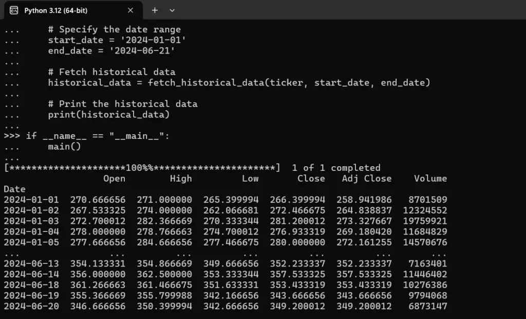
# Print the historical data
print(historical_data)
if __name__ == “__main__”:
main()
- Import Libraries: Import the necessary libraries (yfinance and pandas).
- Fetch Historical Data:
- Use the yf.download function from the yfinance library to fetch historical data.
- The function parameters include the stock ticker, start date, and end date.
- Display Data: Print the historical data, which includes columns for Open, High, Low, Close, Adj Close, and Volume.
The output will be a DataFrame containing the historical stock data with columns for Open, High, Low, Close, Adjusted Close, and Volume. Here’s a sample of what the DataFrame might look like:
Open High Low Close Adj Close Volume
Date
2023-05-01 2389.0000 2400.0000 2370.0000 2385.0000 2385.0000 54321000
2023-05-02 2385.0000 2395.0000 2375.0000 2380.0000 2380.0000 43210000
…
- Date Range: You can specify the desired date range by modifying the start_date and end_date variables.
- Ticker Symbol: Ensure that the stock ticker symbol is accurate. For NSE stocks, the ticker symbol usually ends with .NS (e.g., RELIANCE.NS for Reliance Industries).
If you need to analyze specific time frames (e.g., hourly or minute-wise data), you can adjust the interval parameter in the yf.download function:
def fetch_historical_data(ticker, start_date, end_date, interval=’1d’):
“””Fetch historical data for a specific stock ticker within the given date range and interval.”””
stock_data = yf.download(ticker, start=start_date, end=end_date, interval=interval)
return stock_data
# Example usage for hourly data
historical_data = fetch_historical_data(ticker, start_date, end_date, interval=’1h’)
Valid intervals include 1m (1 minute), 2m, 5m, 15m, 30m, 60m or 1h, 1d, 5d, 1wk, 1mo, 3mo.
This method provides a comprehensive view of historical stock data, enabling thorough analysis and better investment decisions.
Output
Python For Finance
Stock markets are fascinating, they have always been. There are fabulous ways to earn a fortune and need I say loose your money. There are so many indicators that you can utilize to do your next fine investment and it’s easy to get lost in the technical intricacies. The technicalities are tremendous. In this article we will get you started with python for finance. We are using APIs to get financial data. In today’s regard this is going to be with respect to Indian stock market. Let’s get started.
Contents
Step 1: Import Necessary Libraries. 2
Explanation of the Visualization Code: 6
Get High Volatility Shares List 7
Step 1: Install Required Libraries. 7
Getting historical prices of share for a given period of time. 9
Step 2: Fetch Historical Data. 9
Fetching More Detailed Data: 10
Here’s a step-by-step approach you can follow: Let’s say you want to figure out a list of all the share that are listed below Rs 50/- on NSE or National Stock Exchange
- Use a Financial Data API: Utilize a financial data provider API like Alpha Vantage, Yahoo Finance, or similar services that provide stock data.
- Filter the Data: Extract the list of stocks priced below 50 rupees and listed on NSE.
- Analyze for Intraday Performance: Evaluate the stocks based on recent performance indicators, volume, volatility, and other technical indicators.
Here’s how you can proceed with yfinance on your local machine:
- Install yfinance:
pip install yfinance
- Fetch and Filter Data:
importyfinanceasyf
# Example stock tickers (Replace with actual NSE tickers)
nse_stocks = ["YESBANK.NS","IDEA.NS","SUZLON.NS","JPPOWER.NS","RCOM.NS",
"JPASSOCIAT.NS","SOUTHBANK.NS","PUNJLLYOD.NS","GTLINFRA.NS","PNB.NS",
"UNIONBANK.NS","BANKBARODA.NS","IBULHSGFIN.NS","IBREALEST.NS","NBCC.NS",
"RELCAPITAL.NS","RNAVAL.NS","GVKPIL.NS","MTNL.NS","ALOKTEXT.NS",
"TATAPOWER.NS","GMRINFRA.NS","RELINFRA.NS","TTML.NS","JISLJALEQS.NS",
"NCC.NS","SINTEX.NS","DHFL.NS"
]# Fetching stock data
stock_data = yf.download(nse_stocks, period='1d')
# Extracting the current price
current_prices = stock_data['Close'].iloc[-1]
# Filter stocks that are below 50 rupees
filtered_prices = current_prices[current_prices <50]
# Select top 30 stocks
top_30_stocks = filtered_prices.head(30)
print(top_30_stocks)
This script will fetch the current prices for the listed NSE stocks and filter the ones below 50 rupees.
Next we write a detailed Python program to capture trending indicators of shares that can help in analysing data for investment. This example uses various financial indicators like moving averages, RSI, MACD, and Bollinger Bands. Note that for live data fetching and accurate results, you should have access to financial data APIs.
Here’s the detailed Python code:
Step 1: Import Necessary Libraries
First, ensure you have the necessary libraries installed:
pip install yfinance pandas numpy ta
import yfinance as yf
import pandas as pd
import numpy as np
import ta
def fetch_stock_data(ticker, period=’1mo’, interval=’1d’):
“””Fetch historical stock data for the given ticker.”””
stock_data = yf.download(ticker, period=period, interval=interval)
return stock_data
def calculate_moving_averages(df, short_window=20, long_window=50):
“””Calculate short-term and long-term moving averages.”””
df[‘SMA’] = df[‘Close’].rolling(window=short_window, min_periods=1).mean()
df[‘LMA’] = df[‘Close’].rolling(window=long_window, min_periods=1).mean()
return df
def calculate_rsi(df, window=14):
“””Calculate Relative Strength Index (RSI).”””
df[‘RSI’] = ta.momentum.rsi(df[‘Close’], window=window)
return df
def calculate_macd(df):
“””Calculate Moving Average Convergence Divergence (MACD).”””
df[‘MACD’], df[‘MACD_signal’], df[‘MACD_hist’] = ta.trend.macd(df[‘Close’])
return df
def calculate_bollinger_bands(df, window=20, std_dev=2):
“””Calculate Bollinger Bands.”””
df[‘BB_Middle’] = df[‘Close’].rolling(window=window, min_periods=1).mean()
df[‘BB_Upper’] = df[‘BB_Middle’] + std_dev * df[‘Close’].rolling(window=window, min_periods=1).std()
df[‘BB_Lower’] = df[‘BB_Middle’] – std_dev * df[‘Close’].rolling(window=window, min_periods=1).std()
return df
def analyze_stock(ticker):
“””Fetch stock data and calculate technical indicators.”””
df = fetch_stock_data(ticker)
df = calculate_moving_averages(df)
df = calculate_rsi(df)
df = calculate_macd(df)
df = calculate_bollinger_bands(df)
return df
def main():
# Example stock tickers
tickers = [“YESBANK.NS”, “IDEA.NS”, “SUZLON.NS”, “JPPOWER.NS”, “RCOM.NS”]
for ticker in tickers:
print(f”\nAnalyzing {ticker}…”)
df = analyze_stock(ticker)
print(df.tail())
if __name__ == “__main__”:
main()
- Fetch Stock Data:
- fetch_stock_data function uses yfinance to download historical stock data for the given ticker.
- Calculate Moving Averages:
- calculate_moving_averages function calculates short-term (SMA) and long-term (LMA) moving averages. Moving averages help in identifying the trend direction.
- Calculate RSI:
- calculate_rsi function calculates the Relative Strength Index (RSI), which helps in identifying overbought or oversold conditions.
- Calculate MACD:
- calculate_macd function calculates the Moving Average Convergence Divergence (MACD), which is used to identify changes in the strength, direction, momentum, and duration of a trend.
- Calculate Bollinger Bands:
- calculate_bollinger_bands function calculates Bollinger Bands, which are used to measure market volatility and identify overbought or oversold conditions.
- Analyze Stock:
- analyze_stock function fetches the stock data and applies all the technical indicators.
- Main Function:
- The main function runs the analysis for a list of example stock tickers and prints the results.
This code will print the latest values of the calculated indicators for the given stock tickers. You can customize the list of tickers and the parameters for each indicator as needed. For a more comprehensive analysis, we can consider adding more indicators and visualizing the data using libraries like matplotlib or plotly.
Here’s a program to utilize plotly to plot graphs and show stuff visually –
Ensure you have Plotly installed:
pip install plotly
import yfinance as yf
import pandas as pd
import numpy as np
import ta
import plotly.graph_objects as go
def fetch_stock_data(ticker, period=’1mo’, interval=’1d’):
“””Fetch historical stock data for the given ticker.”””
stock_data = yf.download(ticker, period=period, interval=interval)
return stock_data
def calculate_moving_averages(df, short_window=20, long_window=50):
“””Calculate short-term and long-term moving averages.”””
df[‘SMA’] = df[‘Close’].rolling(window=short_window, min_periods=1).mean()
df[‘LMA’] = df[‘Close’].rolling(window=long_window, min_periods=1).mean()
return df
def calculate_rsi(df, window=14):
“””Calculate Relative Strength Index (RSI).”””
df[‘RSI’] = ta.momentum.rsi(df[‘Close’], window=window)
return df
def calculate_macd(df):
“””Calculate Moving Average Convergence Divergence (MACD).”””
df[‘MACD’] = ta.trend.macd(df[‘Close’])
df[‘MACD_signal’] = ta.trend.macd_signal(df[‘Close’])
df[‘MACD_hist’] = ta.trend.macd_diff(df[‘Close’])
return df
def calculate_bollinger_bands(df, window=20, std_dev=2):
“””Calculate Bollinger Bands.”””
df[‘BB_Middle’] = df[‘Close’].rolling(window=window, min_periods=1).mean()
df[‘BB_Upper’] = df[‘BB_Middle’] + std_dev * df[‘Close’].rolling(window=window, min_periods=1).std()
df[‘BB_Lower’] = df[‘BB_Middle’] – std_dev * df[‘Close’].rolling(window=window, min_periods=1).std()
return df
def analyze_stock(ticker):
“””Fetch stock data and calculate technical indicators.”””
df = fetch_stock_data(ticker)
df = calculate_moving_averages(df)
df = calculate_rsi(df)
df = calculate_macd(df)
df = calculate_bollinger_bands(df)
return df
def plot_stock_data(df, ticker):
“””Plot stock data with technical indicators.”””
fig = go.Figure()
# Plot candlestick chart
fig.add_trace(go.Candlestick(
x=df.index,
open=df[‘Open’],
high=df[‘High’],
low=df[‘Low’],
close=df[‘Close’],
name=’Candlesticks’
))
# Plot SMA and LMA
fig.add_trace(go.Scatter(
x=df.index,
y=df[‘SMA’],
line=dict(color=’blue’, width=1.5),
name=’SMA’
))
fig.add_trace(go.Scatter(
x=df.index,
y=df[‘LMA’],
line=dict(color=’red’, width=1.5),
name=’LMA’
))
# Plot Bollinger Bands
fig.add_trace(go.Scatter(
x=df.index,
y=df[‘BB_Upper’],
line=dict(color=’gray’, width=1),
name=’BB Upper’,
opacity=0.5
))
fig.add_trace(go.Scatter(
x=df.index,
y=df[‘BB_Lower’],
line=dict(color=’gray’, width=1),
name=’BB Lower’,
opacity=0.5
))
# Update layout for main plot
fig.update_layout(
title=f'{ticker} Stock Price and Indicators’,
yaxis_title=’Stock Price (INR)’,
xaxis_title=’Date’,
height=800
)
# Create subplot for RSI
fig.add_trace(go.Scatter(
x=df.index,
y=df[‘RSI’],
line=dict(color=’purple’, width=1.5),
name=’RSI’,
yaxis=’y2′
))
# Create subplot for MACD
fig.add_trace(go.Scatter(
x=df.index,
y=df[‘MACD’],
line=dict(color=’orange’, width=1.5),
name=’MACD’,
yaxis=’y3′
))
fig.add_trace(go.Scatter(
x=df.index,
y=df[‘MACD_signal’],
line=dict(color=’green’, width=1.5),
name=’MACD Signal’,
yaxis=’y3′
))
fig.add_trace(go.Bar(
x=df.index,
y=df[‘MACD_hist’],
marker=dict(color=’gray’),
name=’MACD Histogram’,
yaxis=’y3′
))
# Update layout for subplots
fig.update_layout(
yaxis2=dict(
title=’RSI’,
overlaying=’y’,
side=’right’,
position=0.15,
range=[0, 100]
),
yaxis3=dict(
title=’MACD’,
overlaying=’y’,
side=’right’,
position=0.30
)
)
fig.show()
def main():
# Example stock tickers
tickers = [“YESBANK.NS”, “IDEA.NS”, “SUZLON.NS”, “JPPOWER.NS”, “RCOM.NS”]
for ticker in tickers:
print(f”\nAnalyzing {ticker}…”)
df = analyze_stock(ticker)
plot_stock_data(df, ticker)
if __name__ == “__main__”:
main()
Explanation of the Visualization Code:
- Plot Candlestick Chart:
- Uses Plotly’s Candlestick trace to plot the candlestick chart representing the stock’s open, high, low, and close prices.
- Plot Moving Averages:
- Adds Scatter plots for the short-term (SMA) and long-term (LMA) moving averages.
- Plot Bollinger Bands:
- Adds Scatter plots for the Bollinger Bands’ upper and lower bounds.
- Plot RSI and MACD:
- Adds Scatter plots for RSI and MACD, including MACD histogram bars, and creates subplots for better visualization.
- Update Layout:
- Configures the layout of the main plot and subplots for better readability.
- Main Function:
- Analyzes the example stock tickers and plots the data using the defined functions.
Run this code in your local Python environment to visualize the stock data with technical indicators using Plotly. The resulting plots will be interactive, allowing you to zoom in, hover for details, and more.
Get High Volatility Shares List
Here’s another modification to the program we wrote in order to get a list of high volatility shares being traded on NSE whose price is below Rs 100 and are considered good, you can follow these steps:
- Use a Stock Screener: Use a stock screener that allows you to filter stocks based on volatility, price, and other financial metrics.
- Fetch Data Programmatically: You can use APIs or libraries to fetch stock data and calculate volatility.
- Analyze Volatility: Use statistical methods to calculate the volatility of stocks.
- Filter Based on Price: Ensure the stocks are priced below Rs 100.
- Evaluate Quality: Use fundamental and technical indicators to ensure the stocks are of good quality.
Step 1: Install Required Libraries
pip install yfinance pandas numpy ta
Here’s a Python script that fetches stock data, calculates volatility, and filters the stocks based on the criteria:
import yfinance as yf
import pandas as pd
import numpy as np
import ta
def fetch_nse_stock_list():
# Example: This should ideally be a comprehensive list of NSE stocks
# Limited to some examples due to API limitations
nse_stocks = [
“YESBANK.NS”, “IDEA.NS”, “SUZLON.NS”, “JPPOWER.NS”, “RCOM.NS”,
“JPASSOCIAT.NS”, “SOUTHBANK.NS”, “PUNJLLYOD.NS”, “GTLINFRA.NS”, “PNB.NS”,
“UNIONBANK.NS”, “BANKBARODA.NS”, “IBULHSGFIN.NS”, “IBREALEST.NS”, “NBCC.NS”,
“RELCAPITAL.NS”, “RNAVAL.NS”, “GVKPIL.NS”, “MTNL.NS”, “ALOKTEXT.NS”,
“TATAPOWER.NS”, “GMRINFRA.NS”, “RELINFRA.NS”, “TTML.NS”, “JISLJALEQS.NS”,
“NCC.NS”, “SINTEX.NS”, “DHFL.NS”
]
return nse_stocks
def fetch_stock_data(ticker, period=’6mo’, interval=’1d’):
“””Fetch historical stock data for the given ticker.”””
stock_data = yf.download(ticker, period=period, interval=interval)
return stock_data
def calculate_volatility(df):
“””Calculate the volatility of the stock.”””
df[‘Log_Returns’] = np.log(df[‘Close’] / df[‘Close’].shift(1))
volatility = df[‘Log_Returns’].std() * np.sqrt(252) # Annualized volatility
return volatility
def filter_high_volatility_stocks(nse_stocks, max_price=100):
high_volatility_stocks = []
for ticker in nse_stocks:
df = fetch_stock_data(ticker)
if df.empty or df[‘Close’].iloc[-1] > max_price:
continue
volatility = calculate_volatility(df)
if volatility > 0.5: # Example threshold for high volatility
high_volatility_stocks.append({
‘Ticker’: ticker,
‘Price’: df[‘Close’].iloc[-1],
‘Volatility’: volatility
})
return high_volatility_stocks
def main():
nse_stocks = fetch_nse_stock_list()
high_volatility_stocks = filter_high_volatility_stocks(nse_stocks)
# Convert to DataFrame for better readability
df = pd.DataFrame(high_volatility_stocks)
print(df)
if __name__ == “__main__”:
main()
- Fetch NSE Stock List: The fetch_nse_stock_list function provides a list of example NSE stocks. In practice, this list should be comprehensive.
- Fetch Stock Data: The fetch_stock_data function retrieves historical stock data for the given ticker using yfinance.
- Calculate Volatility: The calculate_volatility function computes the annualized volatility based on log returns.
- Filter High Volatility Stocks: The filter_high_volatility_stocks function filters stocks priced below Rs 100 and with high volatility.
- Main Function: The main function runs the process and prints the list of high volatility stocks.
- Threshold for Volatility: The threshold of 0.5 for volatility is an example. Adjust it based on your criteria for high volatility.
- API Limitations: The example uses a limited list of stocks due to API limitations. For a comprehensive analysis, you might need a more extensive list of NSE stocks.
- Data Quality: Ensure the data fetched is accurate and up-to-date. Consider using premium financial data APIs for better reliability.
This script will help you identify high volatility stocks on NSE priced below Rs 100, ensuring they are good for investment based on volatility and price criteria. For further analysis, consider adding fundamental analysis metrics like P/E ratio, market cap, etc.
Getting historical prices of share for a given period of time
To get all historical prices for a particular stock, including open, close, high, and low prices, you can use the yfinance library. This library allows you to download historical market data from Yahoo Finance.
Here’s a step-by-step guide to achieve this:
First, ensure that yfinance is installed:
pip install yfinance
You can use the following Python code to fetch and display historical stock data, including open, close, high, and low prices for a particular stock.
import yfinance as yf
import pandas as pd
def fetch_historical_data(ticker, start_date, end_date):
“””Fetch historical data for a specific stock ticker within the given date range.”””
stock_data = yf.download(ticker, start=start_date, end=end_date)
return stock_data
def main():
# Specify the stock ticker symbol
ticker = ‘RELIANCE.NS’ # Example: Reliance Industries on NSE
# Specify the date range
start_date = ‘2000-01-01’
end_date = ‘2024-06-20’
# Fetch historical data
historical_data = fetch_historical_data(ticker, start_date, end_date)
# Print the historical data
print(historical_data)
if __name__ == “__main__”:
main()
- Import Libraries: Import the necessary libraries (yfinance and pandas).
- Fetch Historical Data:
- Use the yf.download function from the yfinance library to fetch historical data.
- The function parameters include the stock ticker, start date, and end date.
- Display Data: Print the historical data, which includes columns for Open, High, Low, Close, Adj Close, and Volume.
The output will be a DataFrame containing the historical stock data with columns for Open, High, Low, Close, Adjusted Close, and Volume. Here’s a sample of what the DataFrame might look like:
Open High Low Close Adj Close Volume
Date
2023-05-01 2389.0000 2400.0000 2370.0000 2385.0000 2385.0000 54321000
2023-05-02 2385.0000 2395.0000 2375.0000 2380.0000 2380.0000 43210000
…
- Date Range: You can specify the desired date range by modifying the start_date and end_date variables.
- Ticker Symbol: Ensure that the stock ticker symbol is accurate. For NSE stocks, the ticker symbol usually ends with .NS (e.g., RELIANCE.NS for Reliance Industries).
If you need to analyze specific time frames (e.g., hourly or minute-wise data), you can adjust the interval parameter in the yf.download function:
def fetch_historical_data(ticker, start_date, end_date, interval=’1d’):
“””Fetch historical data for a specific stock ticker within the given date range and interval.”””
stock_data = yf.download(ticker, start=start_date, end=end_date, interval=interval)
return stock_data
# Example usage for hourly data
historical_data = fetch_historical_data(ticker, start_date, end_date, interval=’1h’)
Valid intervals include 1m (1 minute), 2m, 5m, 15m, 30m, 60m or 1h, 1d, 5d, 1wk, 1mo, 3mo.
This method provides a comprehensive view of historical stock data, enabling thorough analysis and better investment decisions.
Output
Python For Finance
Stock markets are fascinating, they have always been. There are fabulous ways to earn a fortune and need I say loose your money. There are so many indicators that you can utilize to do your next fine investment and it’s easy to get lost in the technical intricacies. The technicalities are tremendous. In this article we will get you started with python for finance. We are using APIs to get financial data. In today’s regard this is going to be with respect to Indian stock market. Let’s get started.
Contents
Step 1: Import Necessary Libraries. 2
Explanation of the Visualization Code: 6
Get High Volatility Shares List 7
Step 1: Install Required Libraries. 7
Getting historical prices of share for a given period of time. 9
Step 2: Fetch Historical Data. 9
Fetching More Detailed Data: 10
Here’s a step-by-step approach you can follow: Let’s say you want to figure out a list of all the share that are listed below Rs 50/- on NSE or National Stock Exchange
- Use a Financial Data API: Utilize a financial data provider API like Alpha Vantage, Yahoo Finance, or similar services that provide stock data.
- Filter the Data: Extract the list of stocks priced below 50 rupees and listed on NSE.
- Analyze for Intraday Performance: Evaluate the stocks based on recent performance indicators, volume, volatility, and other technical indicators.
Here’s how you can proceed with yfinance on your local machine:
- Install yfinance:
pip install yfinance
- Fetch and Filter Data:
importyfinanceasyf
# Example stock tickers (Replace with actual NSE tickers)
nse_stocks = ["YESBANK.NS","IDEA.NS","SUZLON.NS","JPPOWER.NS","RCOM.NS",
"JPASSOCIAT.NS","SOUTHBANK.NS","PUNJLLYOD.NS","GTLINFRA.NS","PNB.NS",
"UNIONBANK.NS","BANKBARODA.NS","IBULHSGFIN.NS","IBREALEST.NS","NBCC.NS",
"RELCAPITAL.NS","RNAVAL.NS","GVKPIL.NS","MTNL.NS","ALOKTEXT.NS",
"TATAPOWER.NS","GMRINFRA.NS","RELINFRA.NS","TTML.NS","JISLJALEQS.NS",
"NCC.NS","SINTEX.NS","DHFL.NS"
]# Fetching stock data
stock_data = yf.download(nse_stocks, period='1d')
# Extracting the current price
current_prices = stock_data['Close'].iloc[-1]
# Filter stocks that are below 50 rupees
filtered_prices = current_prices[current_prices <50]
# Select top 30 stocks
top_30_stocks = filtered_prices.head(30)
print(top_30_stocks)
This script will fetch the current prices for the listed NSE stocks and filter the ones below 50 rupees.
Next we write a detailed Python program to capture trending indicators of shares that can help in analysing data for investment. This example uses various financial indicators like moving averages, RSI, MACD, and Bollinger Bands. Note that for live data fetching and accurate results, you should have access to financial data APIs.
Here’s the detailed Python code:
Step 1: Import Necessary Libraries
First, ensure you have the necessary libraries installed:
pip install yfinance pandas numpy ta
import yfinance as yf
import pandas as pd
import numpy as np
import ta
def fetch_stock_data(ticker, period=’1mo’, interval=’1d’):
“””Fetch historical stock data for the given ticker.”””
stock_data = yf.download(ticker, period=period, interval=interval)
return stock_data
def calculate_moving_averages(df, short_window=20, long_window=50):
“””Calculate short-term and long-term moving averages.”””
df[‘SMA’] = df[‘Close’].rolling(window=short_window, min_periods=1).mean()
df[‘LMA’] = df[‘Close’].rolling(window=long_window, min_periods=1).mean()
return df
def calculate_rsi(df, window=14):
“””Calculate Relative Strength Index (RSI).”””
df[‘RSI’] = ta.momentum.rsi(df[‘Close’], window=window)
return df
def calculate_macd(df):
“””Calculate Moving Average Convergence Divergence (MACD).”””
df[‘MACD’], df[‘MACD_signal’], df[‘MACD_hist’] = ta.trend.macd(df[‘Close’])
return df
def calculate_bollinger_bands(df, window=20, std_dev=2):
“””Calculate Bollinger Bands.”””
df[‘BB_Middle’] = df[‘Close’].rolling(window=window, min_periods=1).mean()
df[‘BB_Upper’] = df[‘BB_Middle’] + std_dev * df[‘Close’].rolling(window=window, min_periods=1).std()
df[‘BB_Lower’] = df[‘BB_Middle’] – std_dev * df[‘Close’].rolling(window=window, min_periods=1).std()
return df
def analyze_stock(ticker):
“””Fetch stock data and calculate technical indicators.”””
df = fetch_stock_data(ticker)
df = calculate_moving_averages(df)
df = calculate_rsi(df)
df = calculate_macd(df)
df = calculate_bollinger_bands(df)
return df
def main():
# Example stock tickers
tickers = [“YESBANK.NS”, “IDEA.NS”, “SUZLON.NS”, “JPPOWER.NS”, “RCOM.NS”]
for ticker in tickers:
print(f”\nAnalyzing {ticker}…”)
df = analyze_stock(ticker)
print(df.tail())
if __name__ == “__main__”:
main()
- Fetch Stock Data:
- fetch_stock_data function uses yfinance to download historical stock data for the given ticker.
- Calculate Moving Averages:
- calculate_moving_averages function calculates short-term (SMA) and long-term (LMA) moving averages. Moving averages help in identifying the trend direction.
- Calculate RSI:
- calculate_rsi function calculates the Relative Strength Index (RSI), which helps in identifying overbought or oversold conditions.
- Calculate MACD:
- calculate_macd function calculates the Moving Average Convergence Divergence (MACD), which is used to identify changes in the strength, direction, momentum, and duration of a trend.
- Calculate Bollinger Bands:
- calculate_bollinger_bands function calculates Bollinger Bands, which are used to measure market volatility and identify overbought or oversold conditions.
- Analyze Stock:
- analyze_stock function fetches the stock data and applies all the technical indicators.
- Main Function:
- The main function runs the analysis for a list of example stock tickers and prints the results.
This code will print the latest values of the calculated indicators for the given stock tickers. You can customize the list of tickers and the parameters for each indicator as needed. For a more comprehensive analysis, we can consider adding more indicators and visualizing the data using libraries like matplotlib or plotly.
Here’s a program to utilize plotly to plot graphs and show stuff visually –
Ensure you have Plotly installed:
pip install plotly
import yfinance as yf
import pandas as pd
import numpy as np
import ta
import plotly.graph_objects as go
def fetch_stock_data(ticker, period=’1mo’, interval=’1d’):
“””Fetch historical stock data for the given ticker.”””
stock_data = yf.download(ticker, period=period, interval=interval)
return stock_data
def calculate_moving_averages(df, short_window=20, long_window=50):
“””Calculate short-term and long-term moving averages.”””
df[‘SMA’] = df[‘Close’].rolling(window=short_window, min_periods=1).mean()
df[‘LMA’] = df[‘Close’].rolling(window=long_window, min_periods=1).mean()
return df
def calculate_rsi(df, window=14):
“””Calculate Relative Strength Index (RSI).”””
df[‘RSI’] = ta.momentum.rsi(df[‘Close’], window=window)
return df
def calculate_macd(df):
“””Calculate Moving Average Convergence Divergence (MACD).”””
df[‘MACD’] = ta.trend.macd(df[‘Close’])
df[‘MACD_signal’] = ta.trend.macd_signal(df[‘Close’])
df[‘MACD_hist’] = ta.trend.macd_diff(df[‘Close’])
return df
def calculate_bollinger_bands(df, window=20, std_dev=2):
“””Calculate Bollinger Bands.”””
df[‘BB_Middle’] = df[‘Close’].rolling(window=window, min_periods=1).mean()
df[‘BB_Upper’] = df[‘BB_Middle’] + std_dev * df[‘Close’].rolling(window=window, min_periods=1).std()
df[‘BB_Lower’] = df[‘BB_Middle’] – std_dev * df[‘Close’].rolling(window=window, min_periods=1).std()
return df
def analyze_stock(ticker):
“””Fetch stock data and calculate technical indicators.”””
df = fetch_stock_data(ticker)
df = calculate_moving_averages(df)
df = calculate_rsi(df)
df = calculate_macd(df)
df = calculate_bollinger_bands(df)
return df
def plot_stock_data(df, ticker):
“””Plot stock data with technical indicators.”””
fig = go.Figure()
# Plot candlestick chart
fig.add_trace(go.Candlestick(
x=df.index,
open=df[‘Open’],
high=df[‘High’],
low=df[‘Low’],
close=df[‘Close’],
name=’Candlesticks’
))
# Plot SMA and LMA
fig.add_trace(go.Scatter(
x=df.index,
y=df[‘SMA’],
line=dict(color=’blue’, width=1.5),
name=’SMA’
))
fig.add_trace(go.Scatter(
x=df.index,
y=df[‘LMA’],
line=dict(color=’red’, width=1.5),
name=’LMA’
))
# Plot Bollinger Bands
fig.add_trace(go.Scatter(
x=df.index,
y=df[‘BB_Upper’],
line=dict(color=’gray’, width=1),
name=’BB Upper’,
opacity=0.5
))
fig.add_trace(go.Scatter(
x=df.index,
y=df[‘BB_Lower’],
line=dict(color=’gray’, width=1),
name=’BB Lower’,
opacity=0.5
))
# Update layout for main plot
fig.update_layout(
title=f'{ticker} Stock Price and Indicators’,
yaxis_title=’Stock Price (INR)’,
xaxis_title=’Date’,
height=800
)
# Create subplot for RSI
fig.add_trace(go.Scatter(
x=df.index,
y=df[‘RSI’],
line=dict(color=’purple’, width=1.5),
name=’RSI’,
yaxis=’y2′
))
# Create subplot for MACD
fig.add_trace(go.Scatter(
x=df.index,
y=df[‘MACD’],
line=dict(color=’orange’, width=1.5),
name=’MACD’,
yaxis=’y3′
))
fig.add_trace(go.Scatter(
x=df.index,
y=df[‘MACD_signal’],
line=dict(color=’green’, width=1.5),
name=’MACD Signal’,
yaxis=’y3′
))
fig.add_trace(go.Bar(
x=df.index,
y=df[‘MACD_hist’],
marker=dict(color=’gray’),
name=’MACD Histogram’,
yaxis=’y3′
))
# Update layout for subplots
fig.update_layout(
yaxis2=dict(
title=’RSI’,
overlaying=’y’,
side=’right’,
position=0.15,
range=[0, 100]
),
yaxis3=dict(
title=’MACD’,
overlaying=’y’,
side=’right’,
position=0.30
)
)
fig.show()
def main():
# Example stock tickers
tickers = [“YESBANK.NS”, “IDEA.NS”, “SUZLON.NS”, “JPPOWER.NS”, “RCOM.NS”]
for ticker in tickers:
print(f”\nAnalyzing {ticker}…”)
df = analyze_stock(ticker)
plot_stock_data(df, ticker)
if __name__ == “__main__”:
main()
Explanation of the Visualization Code:
- Plot Candlestick Chart:
- Uses Plotly’s Candlestick trace to plot the candlestick chart representing the stock’s open, high, low, and close prices.
- Plot Moving Averages:
- Adds Scatter plots for the short-term (SMA) and long-term (LMA) moving averages.
- Plot Bollinger Bands:
- Adds Scatter plots for the Bollinger Bands’ upper and lower bounds.
- Plot RSI and MACD:
- Adds Scatter plots for RSI and MACD, including MACD histogram bars, and creates subplots for better visualization.
- Update Layout:
- Configures the layout of the main plot and subplots for better readability.
- Main Function:
- Analyzes the example stock tickers and plots the data using the defined functions.
Run this code in your local Python environment to visualize the stock data with technical indicators using Plotly. The resulting plots will be interactive, allowing you to zoom in, hover for details, and more.
Get High Volatility Shares List
Here’s another modification to the program we wrote in order to get a list of high volatility shares being traded on NSE whose price is below Rs 100 and are considered good, you can follow these steps:
- Use a Stock Screener: Use a stock screener that allows you to filter stocks based on volatility, price, and other financial metrics.
- Fetch Data Programmatically: You can use APIs or libraries to fetch stock data and calculate volatility.
- Analyze Volatility: Use statistical methods to calculate the volatility of stocks.
- Filter Based on Price: Ensure the stocks are priced below Rs 100.
- Evaluate Quality: Use fundamental and technical indicators to ensure the stocks are of good quality.
Step 1: Install Required Libraries
pip install yfinance pandas numpy ta
Here’s a Python script that fetches stock data, calculates volatility, and filters the stocks based on the criteria:
import yfinance as yf
import pandas as pd
import numpy as np
import ta
def fetch_nse_stock_list():
# Example: This should ideally be a comprehensive list of NSE stocks
# Limited to some examples due to API limitations
nse_stocks = [
“YESBANK.NS”, “IDEA.NS”, “SUZLON.NS”, “JPPOWER.NS”, “RCOM.NS”,
“JPASSOCIAT.NS”, “SOUTHBANK.NS”, “PUNJLLYOD.NS”, “GTLINFRA.NS”, “PNB.NS”,
“UNIONBANK.NS”, “BANKBARODA.NS”, “IBULHSGFIN.NS”, “IBREALEST.NS”, “NBCC.NS”,
“RELCAPITAL.NS”, “RNAVAL.NS”, “GVKPIL.NS”, “MTNL.NS”, “ALOKTEXT.NS”,
“TATAPOWER.NS”, “GMRINFRA.NS”, “RELINFRA.NS”, “TTML.NS”, “JISLJALEQS.NS”,
“NCC.NS”, “SINTEX.NS”, “DHFL.NS”
]
return nse_stocks
def fetch_stock_data(ticker, period=’6mo’, interval=’1d’):
“””Fetch historical stock data for the given ticker.”””
stock_data = yf.download(ticker, period=period, interval=interval)
return stock_data
def calculate_volatility(df):
“””Calculate the volatility of the stock.”””
df[‘Log_Returns’] = np.log(df[‘Close’] / df[‘Close’].shift(1))
volatility = df[‘Log_Returns’].std() * np.sqrt(252) # Annualized volatility
return volatility
def filter_high_volatility_stocks(nse_stocks, max_price=100):
high_volatility_stocks = []
for ticker in nse_stocks:
df = fetch_stock_data(ticker)
if df.empty or df[‘Close’].iloc[-1] > max_price:
continue
volatility = calculate_volatility(df)
if volatility > 0.5: # Example threshold for high volatility
high_volatility_stocks.append({
‘Ticker’: ticker,
‘Price’: df[‘Close’].iloc[-1],
‘Volatility’: volatility
})
return high_volatility_stocks
def main():
nse_stocks = fetch_nse_stock_list()
high_volatility_stocks = filter_high_volatility_stocks(nse_stocks)
# Convert to DataFrame for better readability
df = pd.DataFrame(high_volatility_stocks)
print(df)
if __name__ == “__main__”:
main()
- Fetch NSE Stock List: The fetch_nse_stock_list function provides a list of example NSE stocks. In practice, this list should be comprehensive.
- Fetch Stock Data: The fetch_stock_data function retrieves historical stock data for the given ticker using yfinance.
- Calculate Volatility: The calculate_volatility function computes the annualized volatility based on log returns.
- Filter High Volatility Stocks: The filter_high_volatility_stocks function filters stocks priced below Rs 100 and with high volatility.
- Main Function: The main function runs the process and prints the list of high volatility stocks.
- Threshold for Volatility: The threshold of 0.5 for volatility is an example. Adjust it based on your criteria for high volatility.
- API Limitations: The example uses a limited list of stocks due to API limitations. For a comprehensive analysis, you might need a more extensive list of NSE stocks.
- Data Quality: Ensure the data fetched is accurate and up-to-date. Consider using premium financial data APIs for better reliability.

This script will help you identify high volatility stocks on NSE priced below Rs 100, ensuring they are good for investment based on volatility and price criteria. For further analysis, consider adding fundamental analysis metrics like P/E ratio, market cap, etc.
Getting historical prices of share for a given period of time
To get all historical prices for a particular stock, including open, close, high, and low prices, you can use the yfinance library. This library allows you to download historical market data from Yahoo Finance.
Here’s a step-by-step guide to achieve this:
First, ensure that yfinance is installed:
pip install yfinance
You can use the following Python code to fetch and display historical stock data, including open, close, high, and low prices for a particular stock.
import yfinance as yf
import pandas as pd
def fetch_historical_data(ticker, start_date, end_date):
“””Fetch historical data for a specific stock ticker within the given date range.”””
stock_data = yf.download(ticker, start=start_date, end=end_date)
return stock_data
def main():
# Specify the stock ticker symbol
ticker = ‘RELIANCE.NS’ # Example: Reliance Industries on NSE
# Specify the date range
start_date = ‘2000-01-01’
end_date = ‘2024-06-20’
# Fetch historical data
historical_data = fetch_historical_data(ticker, start_date, end_date)
# Print the historical data
print(historical_data)
if __name__ == “__main__”:
main()
- Import Libraries: Import the necessary libraries (yfinance and pandas).
- Fetch Historical Data:
- Use the yf.download function from the yfinance library to fetch historical data.
- The function parameters include the stock ticker, start date, and end date.
- Display Data: Print the historical data, which includes columns for Open, High, Low, Close, Adj Close, and Volume.
The output will be a DataFrame containing the historical stock data with columns for Open, High, Low, Close, Adjusted Close, and Volume. Here’s a sample of what the DataFrame might look like:
Open High Low Close Adj Close Volume
Date
2023-05-01 2389.0000 2400.0000 2370.0000 2385.0000 2385.0000 54321000
2023-05-02 2385.0000 2395.0000 2375.0000 2380.0000 2380.0000 43210000
…
- Date Range: You can specify the desired date range by modifying the start_date and end_date variables.
- Ticker Symbol: Ensure that the stock ticker symbol is accurate. For NSE stocks, the ticker symbol usually ends with .NS (e.g., RELIANCE.NS for Reliance Industries).
If you need to analyze specific time frames (e.g., hourly or minute-wise data), you can adjust the interval parameter in the yf.download function:
def fetch_historical_data(ticker, start_date, end_date, interval=’1d’):
“””Fetch historical data for a specific stock ticker within the given date range and interval.”””
stock_data = yf.download(ticker, start=start_date, end=end_date, interval=interval)
return stock_data
# Example usage for hourly data
historical_data = fetch_historical_data(ticker, start_date, end_date, interval=’1h’)
Valid intervals include 1m (1 minute), 2m, 5m, 15m, 30m, 60m or 1h, 1d, 5d, 1wk, 1mo, 3mo.
This method provides a comprehensive view of historical stock data, enabling thorough analysis and better investment decisions.
Output
Overall, Python’s growing presence in finance underscores its significance in shaping the future of financial technology, offering professionals the tools to drive efficiency, innovation, and data-driven insights in an increasingly complex financial landscape.
Curated Reading